Practice how to integrate code and data in Quarto documents
Understand the different output formats from Quarto and how to generate them
Know about generating APA format files with apaquarto and bibtex
This is a short tutorial on using Quarto to mix prose and code together for creating reproducible scientific documents.1
1 This appendix is adapted from a tutorial that Mike Frank and Chris Hartgerink taught together at SIPS 2017.
2 The predecessor to Quarto is R Markdown. Quarto works in much the same way as R Markdown but broadens its functionality substantially—notably it’s not limited to R and can also be used with Python, Javascript, Julia. This tutorial is oriented around Quarto but much of it applies to R Markdown as well, with relatively minor changes in syntax.
3 If you’re interested in the source code for this tutorial, it’s available here.
In short: Quarto allows you to create documents that are compiled with code, producing your next scientific paper.2 This tutorial will help you learn the nuts and bolts of how to do this. This appendix—actually this whole book—is written in Quarto. It’s a very flexible platform for writing nice looking documents.3
C.1 Getting Started
Fire up Rstudio and create a new Quarto document (File > New File > Quarto Document). Don’t worry about the settings, we’ll get to that later.
If you click on the “Render” button (or hit Cmd+Shift+K on Mac or Ctrl+Shift+K on Windows), a document will be generated that includes both content and the output of embedded code, resulting in an HTML file that open in your browser. If RStudio requests you to install packages, click yes and see whether everything works to begin with.
We need that before we teach you more about Quarto. But you should feel good if you get here already, because honestly, you’re about 80% of the way to being able to write basic Quarto documents. It’s that easy.
Noteexercises
Render the Quarto template to PDF (by changing format: html to format: pdf) and Word (format: docx) to ensure that you can get this to work. Isn’t it gratifying? A full list of possible output formats is available here.
C.2 Structure of a Quarto file
A Quarto file contains several parts. Most essential are the header, the body text, and code chunks. When you render the resulting document, you will get the output—text combined with the results of running the code—in one of a number of output formats.
C.2.1 Header
Headers in Quarto files contain some metadata about your document, which you can customize to your liking. Below is a simple example that purely states the title, author name(s), date, and output format.4
4 The header is written in “YAML”, which means “yet another markup language.” You don’t need to know that, and don’t worry about it. Just make sure you are careful with indenting, as YAML does care about that.
The body of the document is where you actually write your reports. This is primarily written in the Markdown format, which is explained in the Markdown syntax section.
The beauty of Quarto is that you can evaluate R code right in the text. To do this, you start inline code with `{r}, type the code you want to run, and close it again with another backtick `. (Usually, this key is below the ESC key or next to the left SHIFT key.)
For example, if you want to have the result of 48 minus 35 in your text, you type `{r} 48-35`, which when rendered becomes 13. Please note that if you return a value with many decimals, it will also print these depending on your settings (for example, `{r} pi` becomes 3.1415927). To change the output number of decimals, you have many options depending on whether you want to set the number of decimals for the whole document or just specific code chunks. See examples here.
C.2.3 Code chunks
In the section above we introduced you to running code inside text, but often you need to take several steps in order to get to the result you need. And you don’t want to do data cleaning in the text! This is why there are code chunks. A simple example is a code chunk loading packages.
First, insert a code chunk by going to Code > Insert Chunk or by pressing Cmd+Option+I in Mac or Ctrl+Alt+I on Windows. Inside this code chunk you can then type for example, library(ggplot2) and create an object x.
If you do not want to have the contents of the code chunk itself to be put into your document, you include #| echo: false as the first line of the code chunk. We can now use the contents from the above code chunk to print results (e.g., “`{r} x`” becomes “2”).
These code chunks can contain whatever you need, including tables, and figures (which we will go into more later). Note that all code chunks regard the location of the source file as the working directory, so when you read in data or otherwise access files, use the relative path to source file.
C.2.4 Output formats
By default, Quarto renders to HTML, the standard format of web pages. These output files are visible in the RStudio viewer and in any web browser. These files can be shared on the web and are a great way to provide the outputs of your research to collaborators (e.g., sharing intermediate analytic results).
Through a program called pandoc, Quarto can also render to Microsoft Word’s docx format. This functionality can be very useful for sharing editable write-ups with collaborators (see below).
Finally, rendering to PDF is useful for creating publication manuscripts, or other research outputs that require a specific static format. If you want to create PDFs from Quarto you need a installation on your computer. (, or tex for short, is a powerful typesetting system). Many tex installations are available. One recent possibility is TinyTEX, a minimal tex installation made for R users. Or if you want a full install, try MikTeX for Windows, MacTeX for Mac, or TeX Live for Linux.
C.3 Markdown syntax
Markdown is one of the simplest document languages around, that is an open standard and can be converted into .tex, .docx, .html, .pdf, etc. This is the main workhorse of Quarto and is very powerful. You can learn Markdown in five minutes. Other resources include this tutorial, and the help page that pops up if you go to Help > Markdown Quick Reference in RStudio.
These are the basics:
It’s easy to get *italic* and **bold** (or equivalently _italic_ and __bold__).
You can get headings using # heading1 for first level, ## heading2 for second-level, and ### heading3 for third level. Make sure you leave a space after the #!
Lists are delimited with * at the start of each entry (for unordered lists) or any digit at the start of the entry (for ordered lists).
You can write links by writing [here's my link](http://foo.com).
The great thing about Markdown is that it’s designed to be easy to read and is used in many platforms, e.g. GitHub, OSF, Slack, and many wikis.
C.4 Chunk options
At the start of each code chunk, you can include a variety of options that affect how the chunk is handled by Quarto. For example, the echo: false option suppresses the code from appearing in the output:
```{r}2+2```
#> [1] 4
Chunk options to are often added to code chunks include:
code does or doesn’t display inline (echo option)
warnings and messages are suppressed (warning and message option)
computations are cached (cache option)
Caching can be very helpful for large files, but can also cause problems when there are external dependencies that change. You can also set chunk options in the YAML header, which will apply to all chunks in the document unless overwritten in individual chunks.
There are also many other chunk options not necessarily related to code execution, which can be set in the same way as above for individual chunks, and specified at the document-level in YAML under knitr, e.g.:
---knitr:opts_chunk:comment:"#>"---
C.5 Headings, figures, and tables
We’re going to want some more libraries loaded for the sections below.
library(knitr)library(ggplot2)library(broom)
C.5.1 Headings
As mentioned above, headings are specified in Markdown using # level 1 heading, ## level 2 heading, etc.
Noteexercises
Outlining using headings is a really great way to keep things organized! Try making a bunch of headings, and then rendering your document.
To show off your headings from the previous exercise, add a table of contents. Go to the YAML header of the document, and add an option under format. You want it to look like this (indentation must to be correct):
format:html:toc:true
C.5.2 Figures
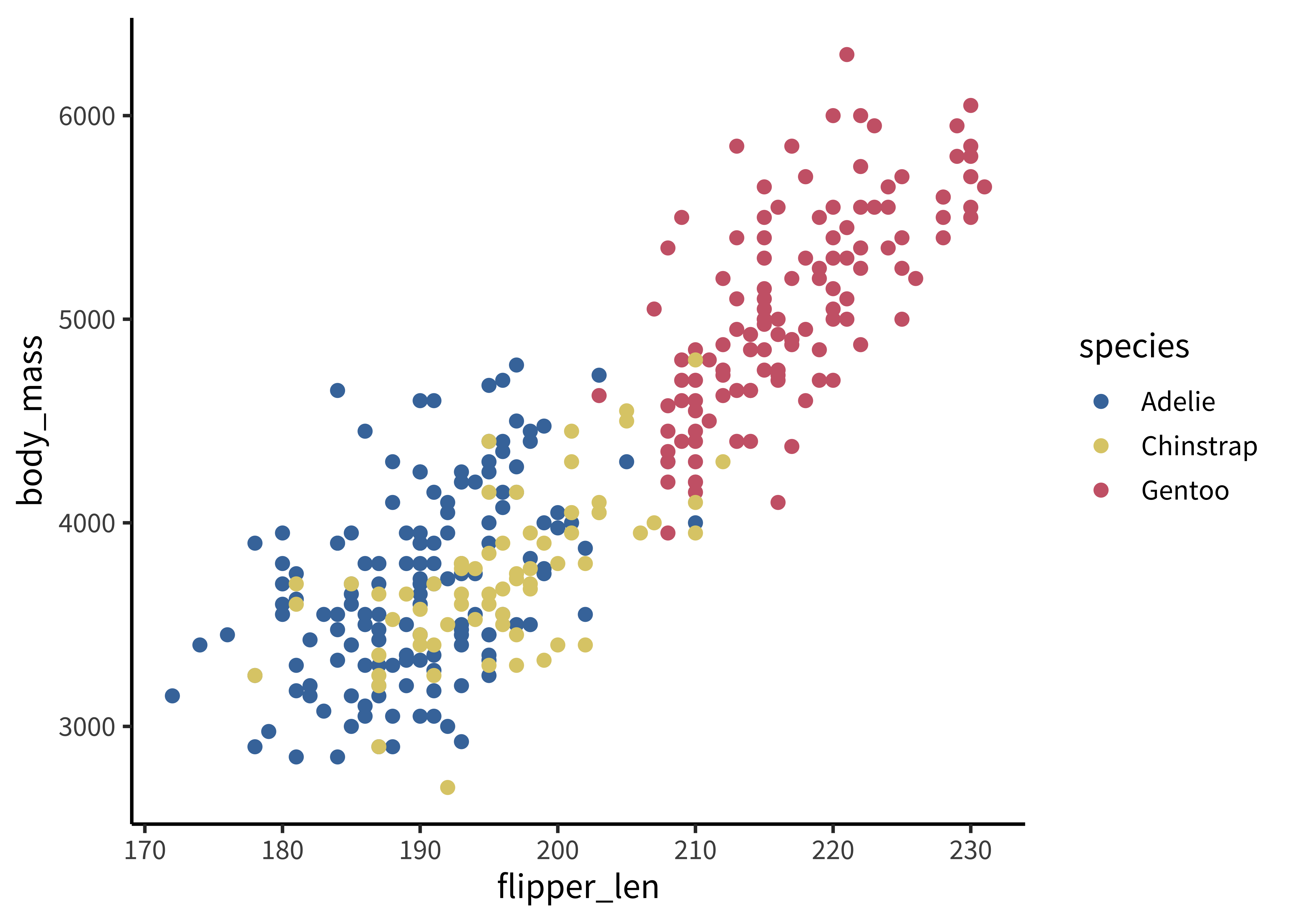
It’s really easy to include plots, like this one. (Using the penguins dataset that comes with R).
All you have to do is output the plot and it will be rendered straight into the text. Chunk options can be used to control the figure’s size and add a caption and cross-referenceable label.
```{r}#| fig-cap: "Body mass (g) vs. flipper length (mm) for three species of penguins."#| label: fig-penguins#| fig-width: 6#| fig-height: 3ggplot(penguins, aes(x = flipper_len, y = body_mass, colour = species)) +geom_point()```
Figure C.1: Body mass (g) vs. flipper length (mm) for three species of penguins.
External graphics can also be included, as follows (the part in {} is optional):
There are many ways to make good-looking tables using Quarto, depending on your display purpose.
The knitr package comes with the kable() function. It’s versatile and makes perfectly reasonable tables across a variety of output formats. It also has a digits argument for controlling rounding.
The flextable package provides a framework for creating tables for reporting/publication and has more features and customization than kable().
For HTML tables specifically, there is the DT package, which provides datatable()—these are pretty and interactive JavaScript-based tables that you can click on and search in. Not great for static documents though.
For APA manuscripts or other PDFs, it can also be helpful to use the xtable package, which creates very flexible LaTeX tables. These can be tricky to get right but they are completely customizable provided you want to google around and learn a bit about LaTeX.
We recommend starting with kable(). For example:
```{r}kable(head(penguins), digits =1)```
species
island
bill_len
bill_dep
flipper_len
body_mass
sex
year
Adelie
Torgersen
39.1
18.7
181
3750
male
2007
Adelie
Torgersen
39.5
17.4
186
3800
female
2007
Adelie
Torgersen
40.3
18.0
195
3250
female
2007
Adelie
Torgersen
NA
NA
NA
NA
NA
2007
Adelie
Torgersen
36.7
19.3
193
3450
female
2007
Adelie
Torgersen
39.3
20.6
190
3650
male
2007
Noteexercises
Using the penguins dataset, insert a table and a plot of your choice into your Quarto document. If you’re feeling uninspired, try hist(penguins$body_mass).
C.5.4 Statistics
It’s also really easy to include statistical tests of various types. One option is to use the broom package, which formats the outputs of various tests really nicely. Paired with kable() you can make very simple tables in just a few lines of code. For example:
Cleaning these tables up for publication can take some work. For example, we’d need to rename a bunch of fields to make this table have the labels we wanted (e.g., to turn flipper_len into Flipper length (mm)).
We often need APA-formatted statistics to be printed in text, though. A good approach is to compute them first, and then print them inline. First, we’d run something like this:
There is a statistically significant difference in bill length between Chinstrap and Gentoo penguins (\(t(129.22) = 2.71\), \(p = 0.008\)).
We did this using inline code blocks, e.g. `{r} round(ts$parameter, 2)`.
Rounding \(p\)-values can occasionally get you in trouble. It’s very easy to have an output of \(p = 0\) when in fact \(p\) can never be exactly equal to 0. Nonetheless, this can help you prevent the kinds of rounding errors that would get picked up by software like statcheck.
C.6 Writing APA-format papers
The end-game of reproducible research is to render your entire paper into a submittable APA-style writeup. Managing APA format is a pain in the best of times. The apaquarto extension allows you to simplify this task by rendering your manuscript directly from Quarto.5
5 The corresponding package for R Markdown is papaja.
To use apaquarto, first install the quarto R package (install.packages("quarto")). Make a folder for where your document and associated files will go, set it to be your working directory (Session > Set Working Directory), and then run:
quarto::quarto_use_template("wjschne/apaquarto")
A bunch of files should get created and your document is ready to go!
Noteexercises
Follow the steps above to set an apaquarto document. Render it (to one or more of the available formats), and look at how awesome it is.Try pasting in your figure and table from your other document (don’t forget any libraries you need to make it run).
C.7 Bibiographic management
Managing a bibliography by hand is a lot of work. Letting software do this for you is much easier. In Quarto it’s possible to include references using bibtex, by using @ref syntax.
It’s simple. You put together a set of paper citations in a bibtex file—then when you refer to them in text, the citations pop up formatted correctly, and they are also put in your bibliography. As an example, @nuijten2016 results in the in text citation “Nuijten et al. (2016)”, or cite them parenthetically with [@nuijten2016](Nuijten et al. 2016). See the Quarto docs more citation options.
How do you make your bibtex file? You can do it by hand but this is a pain. One option for managing references is bibdesk, which integrates with google scholar.6citr is an R package that provides an easy-to-use RStudio addin that facilitates inserting citations. The addin will automatically look up the Bib(La)TeX-file(s) specified in the YAML front matter. The references for the inserted citations are automatically added to the documents reference section. Once citr is installed (install.packages("citr")) and you have restarted your R session, the addin appears in the menus and you can define a keyboard shortcut to call the addin.
6 Many other options are possible. For example, some of us use Zotero frequently as well.
C.8 Collaboration
How do we collaborate using Quarto? There are lots of different workflows that people use. Here are a few:
The lead author makes a Git repository with the Quarto document in it. Others read the rendered PDF and send text comments or PDF annotations and the lead makes modifications to the source file accordingly.7 This workflow works well when the lead author is relatively experienced and wants to keep control of the manuscript without too much line-by-line rewriting.
The lead author makes a repository as above, but coauthors collaborate either by pushing changes to the Git repository, either to the main branch or by creating pull requests. This workflow works well when the authors are all fairly Git-savvy, and can be great for quickly writing different parts in parallel because of Git’s automatic merging.8
The authors work collaboratively together in an editor like Google Docs, Word, or Overleaf. (We favor cloud platforms rather than emailing back and forth, for all the reasons discussed in chapter 13). Once the substantive text sections have converged, the lead author puts that text back into the Quarto document and adds references and other programmatic elements. This workflow is good for very collaborative introduction writing when coauthors don’t use Git or Markdown. This workflow is a little clunky, but not too bad. And critically, all the figures and numbers get rendered fresh when you render, so nothing can get accidentally altered during the editing process.
The lead author renders the results section from Quarto, then writes text in the resulting Word document (or uploads it to Google Docs). This workflow is closest to the “old way” that many people are used to, but runs the biggest risk of errors getting introduced and propagated forward, since it’s not possible to re-render the whole document from scratch. If someone makes changes to the results section, it’s critical to propagate these back to the source file and keep the two in sync.
7 Dropbox has good PDF annotation tools for writing comments on specific lines of text.
8 We wrote this book using the all-github workflow, and it was pretty good, modulo some merge conflicts.
In sum, there are lots of ways to collaborate—the best thing is to talk with your coauthors to select one that works for the group.
C.9 Quarto: Chapter summary
Quarto is a great way to write reproducible papers. It is not too tricky to learn, and once you master it you can save time by reformatting quickly and automatically, managing your bibliography automatically, and even creating nice web-compatible documents.
Nuijten, Michèle B., Chris H J Hartgerink, Marcel A L M van Assen, Sacha Epskamp, and Jelte M Wicherts. 2016. “The Prevalence of Statistical Reporting Errors in Psychology (1985–2013).”Behavior Research Methods 48 (4): 1205–26.