5 Estimation
- Estimate the causal effect of a manipulation
- Discuss differences between frequentist and Bayesian estimation
- Reason about standardized effect sizes and their strengths and weaknesses
- Quantify the relationship between variables
In every quantitative paper we read, every quantitative talk we attend, and every quantitative article we write, we should all ask one question: what is the estimand? The estimand is the object of inquiry—it is the precise quantity about which we marshal data to draw an inference. Yet, too often social scientists skip the step of defining the estimand. Instead, they leap straight to describing the data they analyze and the statistical procedures they apply. Without a statement of the estimand, it becomes impossible for the reader to know whether those procedures were appropriate.
—Lundberg, Johnson, and Stewart (2021, 532)
In part I of this book, our goal was to set up some of the theoretical ideas that motivate our approach to experimental design and planning. We introduced our thesis, namely that experiments are about measuring causal effects, and began discussing our themes: transparency, measurement precision, bias reduction, and generalizability.
Now, in part II—treating statistical topics—we will integrate these ideas with an analytic toolkit for estimating effects and quantifying their size (this chapter), making inferences about how these estimates relate to a population (chapter 6), and building models for estimation and inference in more complex settings (chapter 7). Although this book does not provide an extensive treatment of statistics, we hope that these chapters provide a foundation—and an opinionated perspective—for beginning the statistical analysis of your experimental data, with a focus on measurement precision.
The Lady Tasting Tea
The birth of modern statistical inference arose from the age-old conundrum of how to best make a cup of tea. The statistician Ronald Fisher was apparently at an afternoon tea party when a lady declared that she could tell the difference when tea was added to milk vs milk to tea. Rather than taking her at her word, Fisher devised an experimental and data analysis procedure to test her claim.
The lady would have to judge a set of six new cups of tea and sort them into milk-first vs tea-first sets. Her data would then be analyzed to determine whether her level of correct choice exceeded that expected by chance. While this process now sounds like a quotidian experiment that might be done on a cooking reality show, it seems unremarkable in hindsight only because it set the standard for the way science was done going forward.
The important and unusual element of the experiment was its treatment of potential design confounds such which cup of tea was prepared first, which cup of tea was presented first, or the material that the cups were made out of. Prior experimental practice would have been to try to equate all of the cups as closely as possible, decreasing the influence of confounds. Fisher recognized that this strategy was insufficient because of the presence of unobserved confounders. Only by randomizing all other aspects of the experiment could he make strong causal inferences about the treatment (milk then tea vs tea then milk). We discussed the causal power of random assignment in chapter 1—the Lady Tasting Tea experiment is a key touchstone in the popularization of randomized experiments!
5.1 Estimating a quantity
If experiments are about estimating effects, how do we actually use our experimental data to make these estimates? For our example we’ll design a more modern version of Fisher’s1 experiment (figure 5.1).
1 An important piece of context for the work of Ronald Fisher, Karl Pearson, and other early pioneers of statistical inference is that they were strong proponents of eugenics. Fisher was the founding chairman of the Cambridge Eugenics Society. Pearson was perhaps even worse, an avowed Social Darwinist who believed fervently in eugenic legislation. Irrespective of their scientific content (which was often incorrect), these views are morally repugnant.
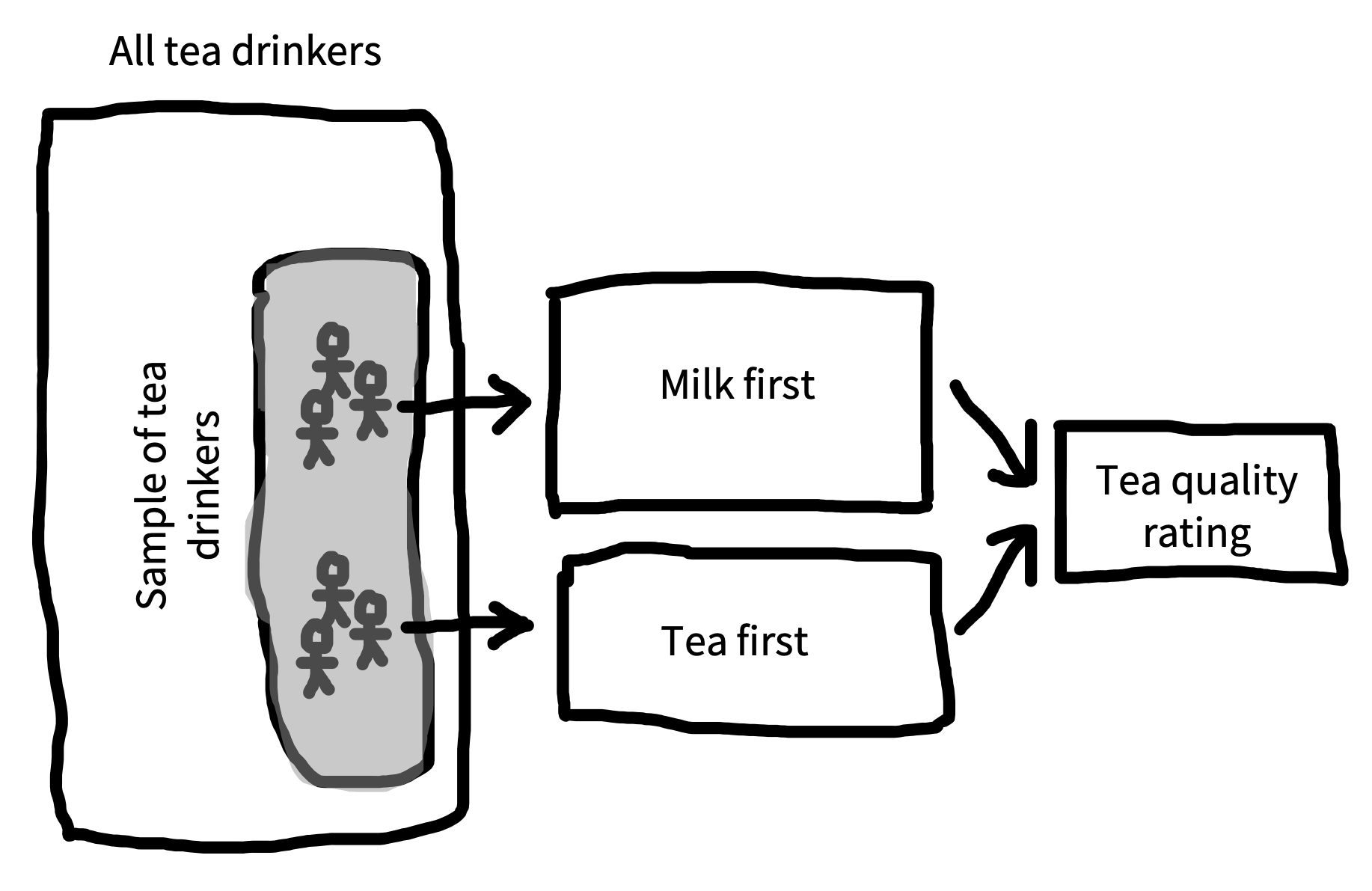
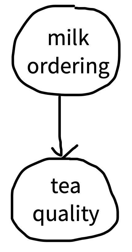
Our causal theory is that the tea quality is affected by milk-tea ordering, so we’ll test that by rating tea quality both milk-first and tea-first, represented by a DAG like the one in figure 5.2. Our intended population to generalize to is the set of all tea drinkers, and toward that goal we sample a set of tea drinkers. In practice, we might do a field trial in a cafe in which we approach patrons and ask them to participate in our experiment in exchange for a free cup of tea. Although this sample size is almost certainly too small to get precise estimates, for the purpose of this example, we’ll sample 18 tea drinkers—nine in each condition.
2 Technically, randomized experiments were not invented by Fisher. Perhaps the earliest example of a (somewhat) randomized experiment was a trial of scurvy treatments in the 1700s (Dunn 1997). Peirce and Jastrow (1884) also report a strikingly modern use of randomized stimulus presentation (via shuffling cards). Nevertheless, Fisher’s statistical work popularized randomized experiments throughout the sciences, in part by integrating them with a set of analytic methods.
3 Right now we’re going to assume that our ratings are just simple numerical values and not worry about the fact that they come from a rating scale that is bounded (e.g., can’t go above 7). If you’re curious about Likert scales (the name for discrete numerical rating scales; pronounced LICK-ert), we’ll talk a bit more about them in chapter 8.
As our manipulation, we follow Fisher in randomly assigning participants (who of course should give consent to participate) to one of two conditions: milk-first or tea-first.2 This is a between-participants design, so each participant gets only one cup of tea. They receive their cup of tea and taste it. Then, as our measure, we ask for a rating of the tea on a continuous scale from 1 (terrible) to 7 (delicious).3
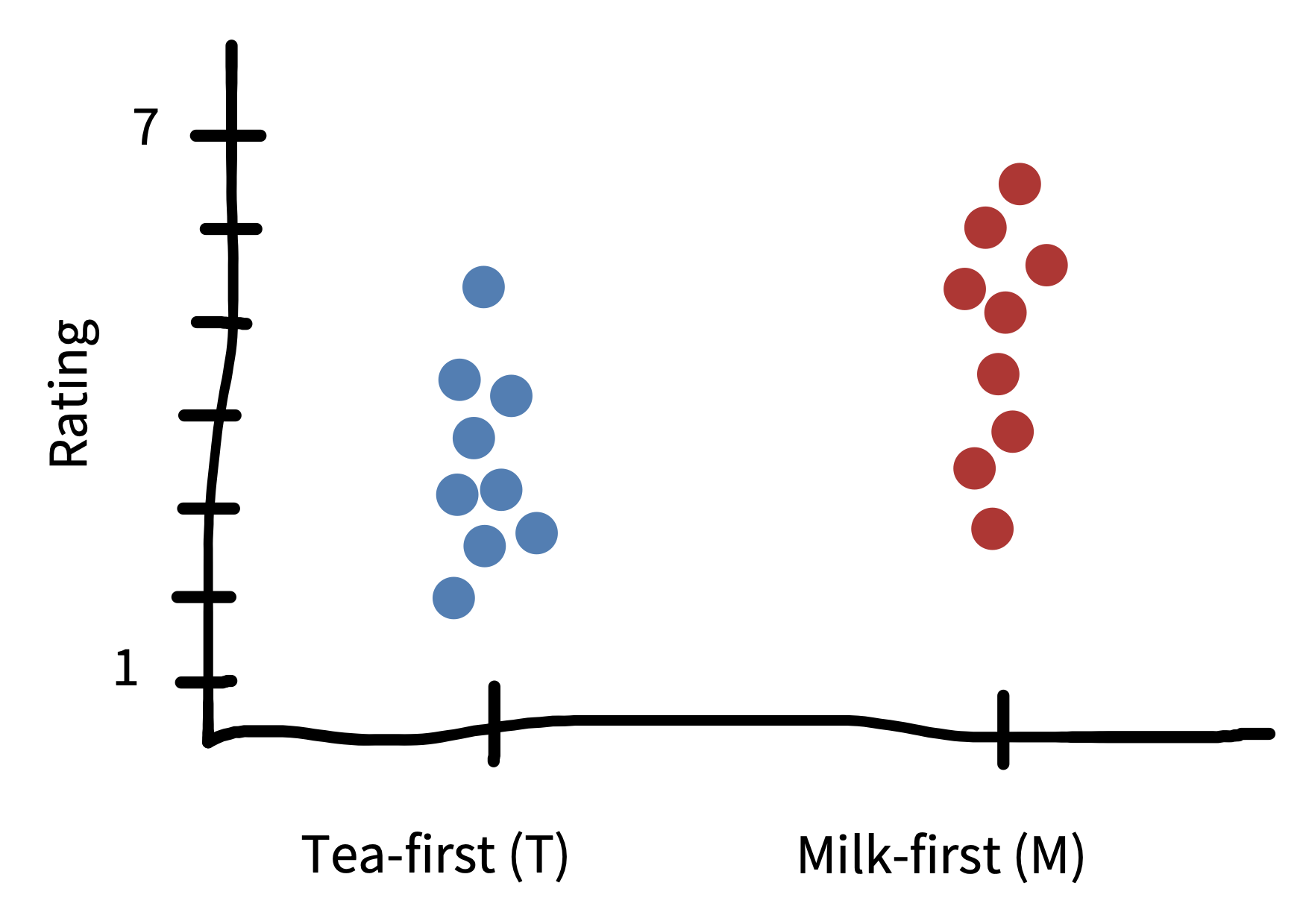
An example dataset from our experiment is shown in figure 5.3. Eventually, we’ll want to estimate the effect of milk-first preparation on quality ratings (our effect of interest). But for now, our goal will be to estimate the quality of the tea when it is milk-first (which some data suggest is actually the better way, at least for British tea drinkers; Kennedy 2003). More formally, we want to use our sample of nine milk-first tea judgments to estimate a number that we can’t directly observe, namely the true perceived quality of all possible milk-first cups. We’ll call this number a population parameter for reasons that will become clear soon.
We’ll try to go easy on notation, but some amount will hopefully make things clearer. We’ll use \(\theta_{M}\) (“theta”) to denote the parameter we want to estimate (the population parameter) and \(\widehat{\theta}_{M}\) for sample estimate.4
4 Statisticians use “hats” like this to denote estimates from a specific sample. One way to remember this is that the “person in the hat” is wearing a hat to dress up as the actual quantity.
5.1.1 Maximum likelihood estimation
Okay, you are probably saying, if we want our estimate of milk-first quality, shouldn’t we just take the average rating across the nine cups of milk-first tea? The answer is yes. But let’s unpack that choice: taking the sample mean as our estimate \(\widehat{\theta}_{M}\) is an example of an estimation approach called maximum likelihood estimation. In general terms, maximum likelihood estimation is a two-step process.
First, we assume a model for how the data were generated.5 This model is specified in terms of certain population parameters. In our example, the model is as simple as they come: we just assume there is some average level of tea quality and that the measurements vary around it. Let’s take a look at the data from the milk-first condition, shown in figure 5.4. Our observations are clustered around the mean, but they also show some variation. Some are higher and some are lower. Variation of this type is a feature of every data set. This variation can be summarized via a probability distribution, a mathematical entity that describes the properties of possible datasets.
5 This sense of “model” is actually a formal instantiation of the type of causal model we discussed in chapter 1. As you get deeper into causal modeling, typically what you do is define a causal “story” for the statistical process that generated a dataset, using both DAGs and the kinds of probability distributions we will define below.
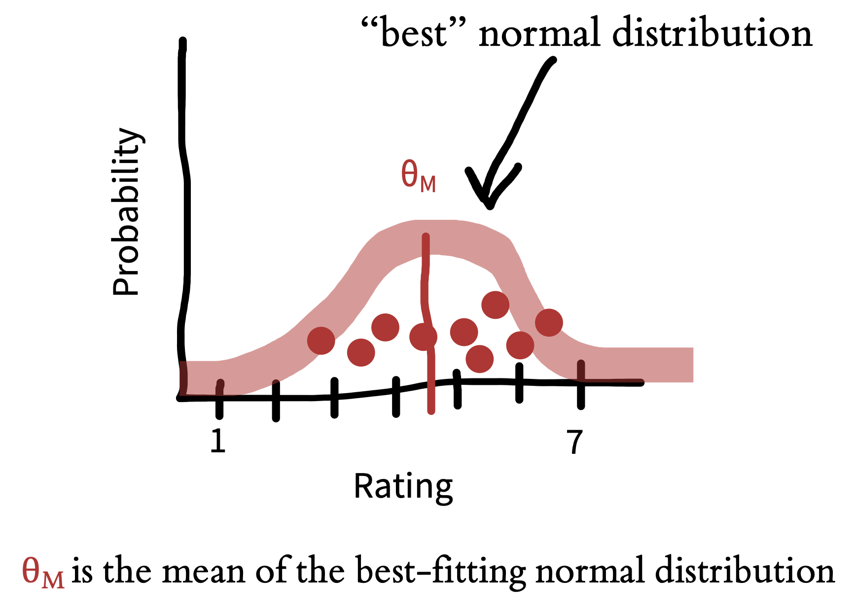
The only probability distribution we’ll discuss here is the ubiquitous normal distribution (also sometimes called a “Gaussian distribution”). A normal distribution has two parameters (numbers that define its shape): a mean and a standard deviation. These two parameters define the shape of the curve. The mean (\(\theta_M\)) describes where its center goes, and the standard deviation describes how wide it is. Technically, the mean is the expected value for new samples from the distribution. Our best guess about the value of these new samples is that they are at the mean. We can write this more formally by introducing \(E[M]\) to denote the expectation of the variable \(M\).
The standard deviation \(\sigma_M\) is then a way of describing the expected variation in these samples. A bigger standard deviation means that we expect samples to be on average further from the mean. We can write this formally as \(\sigma_M = \sqrt{E[(M - \theta_M)^2]}\): the standard deviation is the expected absolute distance between individual samples and the mean, with the square and square root being necessary to compute distance.
Using a probability distribution to describe our dataset gives us a way of summarizing our observations through the parameters of the distribution and encoding an assumption about what future observations might look like. How do we fit a normal distribution to our data? We try to find the values of the population parameters that make our observed data as likely as possible. Let’s start with the mean.
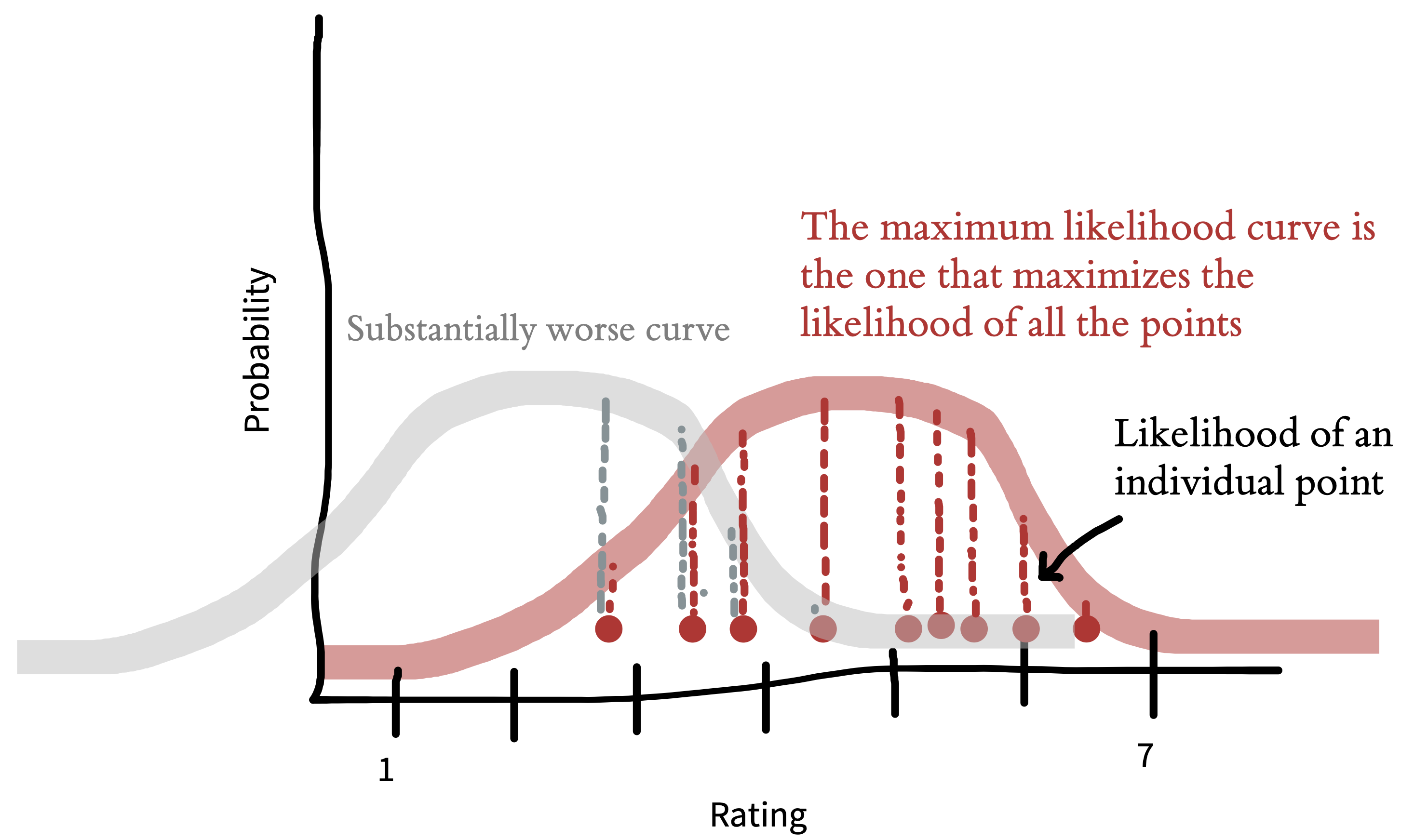
For example, if our sample mean is \(\widehat{\theta}_{M} = 4.5\), what underlying value of \(\theta_{M}\) would make these data most likely to occur? Well, suppose the underlying parameter were \(\theta_{M}=2.5\). Then it would be pretty unlikely that our sample mean would be so much bigger. So, \(\widehat{\theta}_{M}=2.5\) is a poor estimate of the population parameter based on these data (figure 5.5). Conversely, if the parameter were \(\theta_{M}=6.5\), it would be a bit unlikely that our sample mean would be so much smaller. The value of \(\widehat{\theta}_{M}\) that makes these data most likely is \(4.5\) itself: the sample mean! That is why the sample mean in this case is the maximum likelihood estimate.
5.1.2 Bayesian estimation
The maximum likelihood estimation example above represents a common approach to estimating parameters, where the researcher completely puts aside their prior expectations about what these values might be. This approach is an example of a frequentist statistical approach, an approach that focuses on the long-run performance of estimation procedures.
Often this approach makes sense, especially when we have no prior expectations about the values we are estimating. But sometimes we do have relevant beliefs about the value. For example, before we perform our tea experiment, we don’t know exactly what \(\theta_{M}\) will be, but it seems a bit unlikely that tea would be consistently rated as either horrible (1) or perfect (7). We have what you might call weak prior expectations about the kinds of ratings we’ll receive.
These kind of expectations are most useful when we have a very small amount of data. Remember that our goal is to estimate a population parameter using the sample data, and small data sets can be rather noisy. Taking into account our prior expectations can help to temper the influence of noise. For example, if our very first participant in the experiment rated their tea as terrible, we wouldn’t want to jump to the conclusion that the tea was actually bad. Instead, we might speculate that the participant was having a bad day or had just brushed their teeth. On the other hand, if all of our participants gave bad ratings to their tea, the data would be more persuasive; in that case, we might want to tell the cafe that they are serving substandard tea. The extent to which our prior expectations should moderate our conclusions should vary with the amount of sample data; with only a little data, our prior expectations should have more influence, but as we gather more, we should put greater weight on the data.
How do we quantify this trade-off between our prior expectations and our current observations? We can do this via Bayesian estimation of \(\widehat{\theta}_{M}\). Bayesian estimation provides a principled framework for integrating prior beliefs and data. These estimation techniques can be very helpful in cases where data are sparse or prior beliefs are strong.
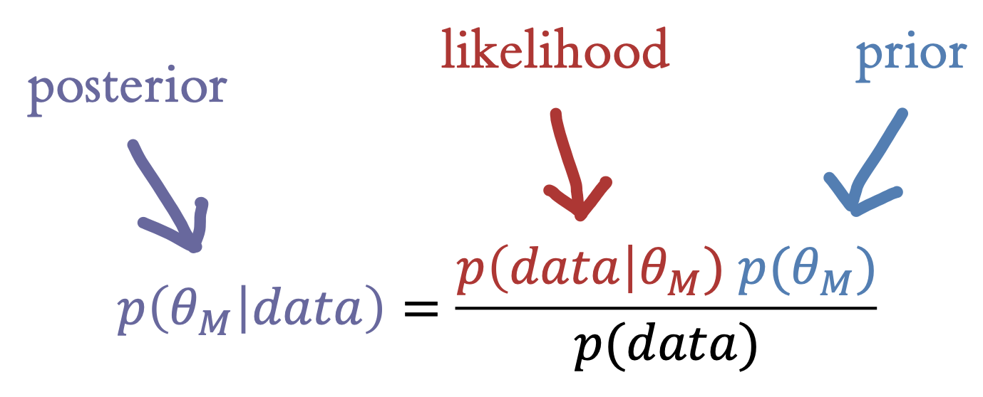
In Bayesian estimation, we observe some data \(d\), consisting of the set of responses in the experiment. Now we can use Bayes’s rule, a tool from basic probability theory, to estimate this number (figure 5.6). Each part of this equation has a name, and it’s worth becoming familiar with them. The thing we want to compute, \(p(\theta_{M} |\text{data})\), is called the posterior probability—it tells us what we should believe about the population parameter on tea quality, given the data we observed.6
6 We’re making the posterior purple to indicate the combination of likelihood (red) and prior (blue).
7 Speaking informally, likelihood is just a synonym for probability, but in Bayesian estimation, likelihood is a technical term specifically referring to probability of the data given our hypothesis. This ambiguity can get a bit confusing.
The first part of the numerator is \(p(\text{data}|\theta_{M})\), the probability of the data we observed given our hypothesis about the participant’s ability. This part is called the likelihood.7 This term tells us about the relationship between our hypothesis and the data we observed—so, if we think the tea is of high quality (say \(\theta_{M} = 6.5\)), then the probability of observing a bunch of low-quality ratings will be fairly low.
The second term in the numerator, \(p(\theta_{M} )\), is called the prior. This term encodes our beliefs about the likely distribution of tea quality. Intuitively, if we think that the tea is likely high quality, we should require more evidence to be convinced it’s bad. In contrast, if we think it’s probably bad, a few low ratings might serve to convince us.
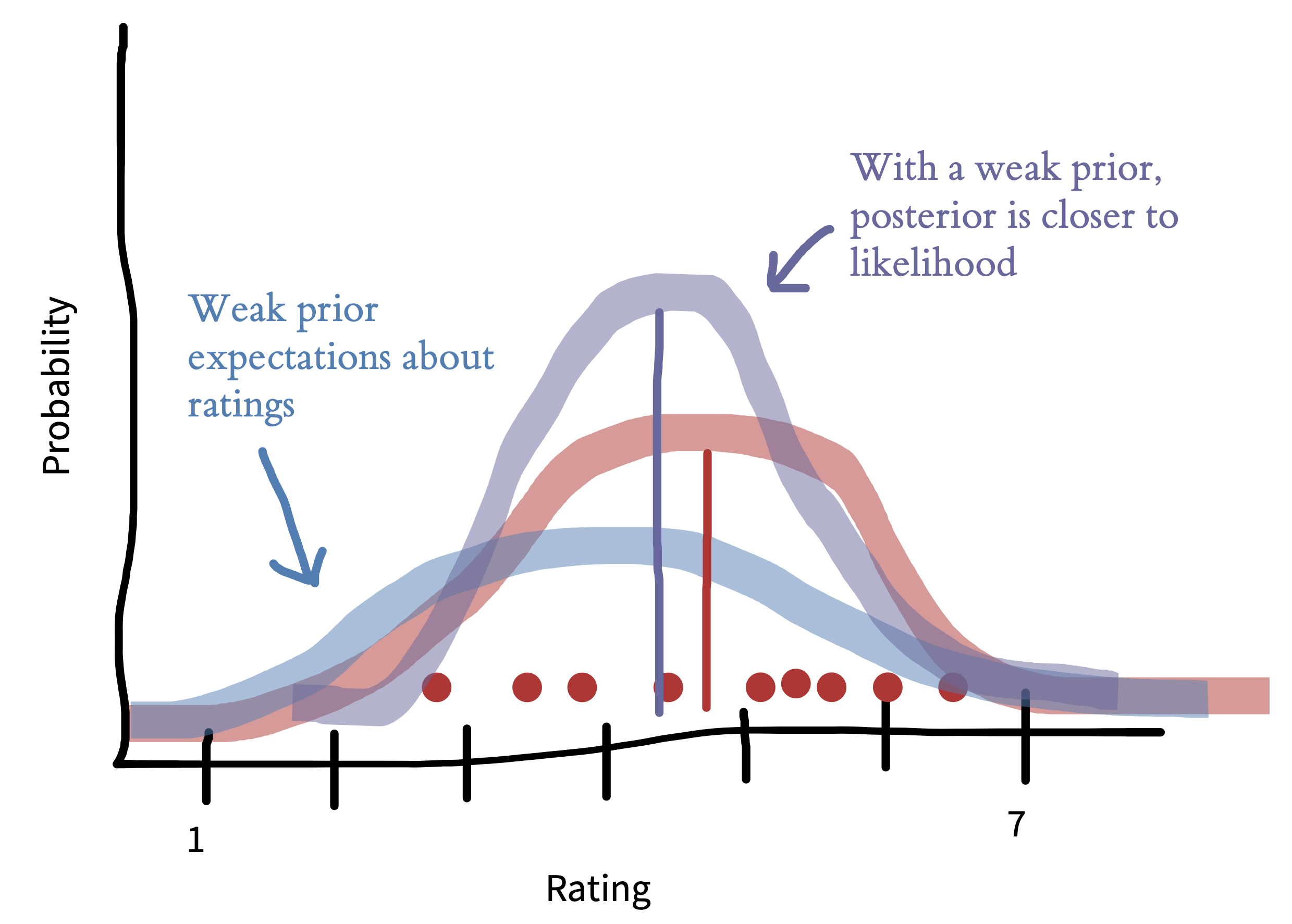
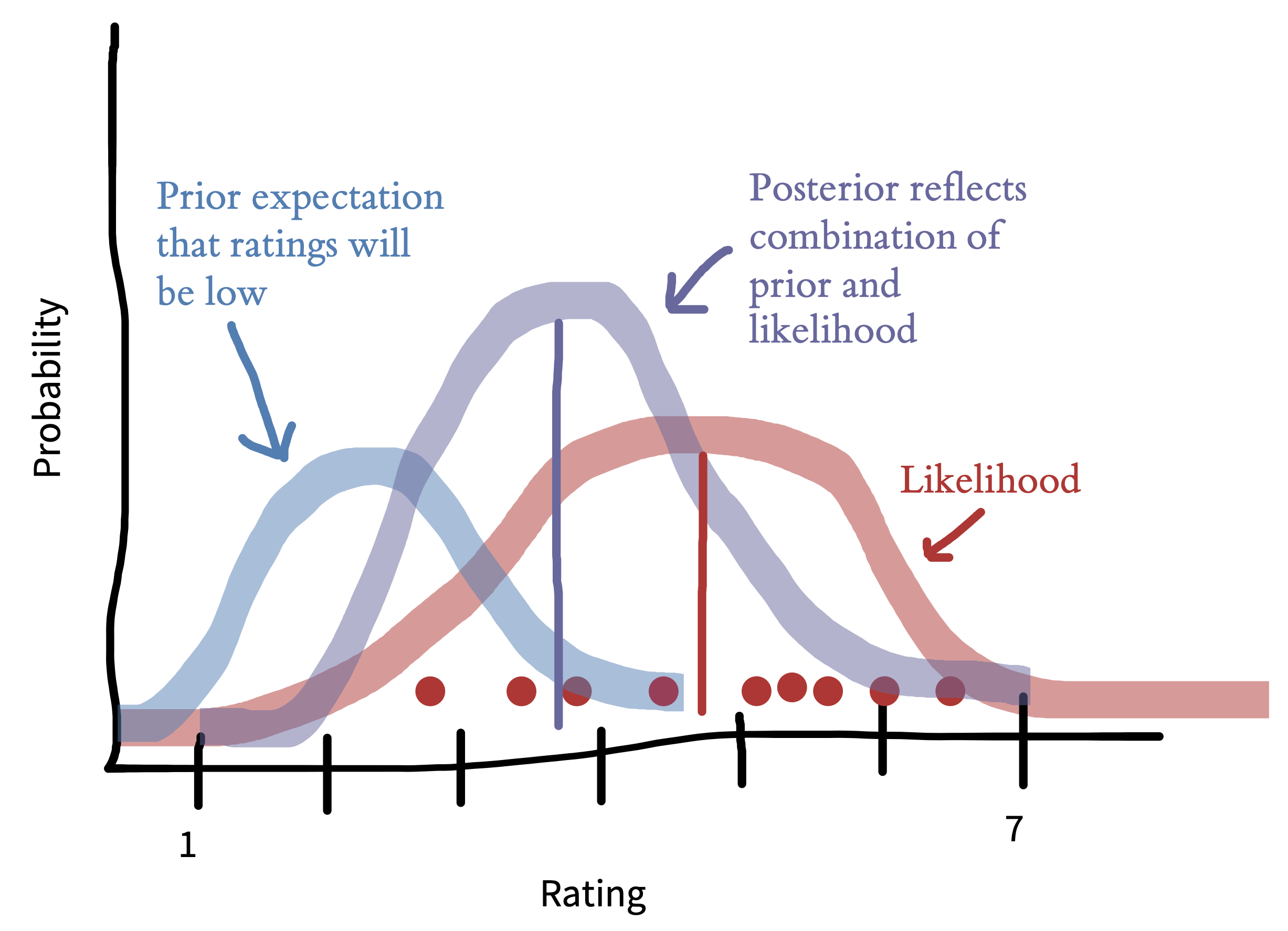
Figure 5.7 gives an example of the combination of prior and data. In this example, we look at what difference the prior makes after observing 9 ratings. If we go in assuming that the tea is likely to be bad, the posterior mean (purple line) will be pushed downward relative to the maximum likelihood estimate (red line). This prior is operating only over on ratings—estimates of tea quality. Later on when we talk about comparing milk-first and tea-first ratings to get an estimate of the experimental effect, we could consider putting a prior on tea discrimination (e.g., the experimental effect).
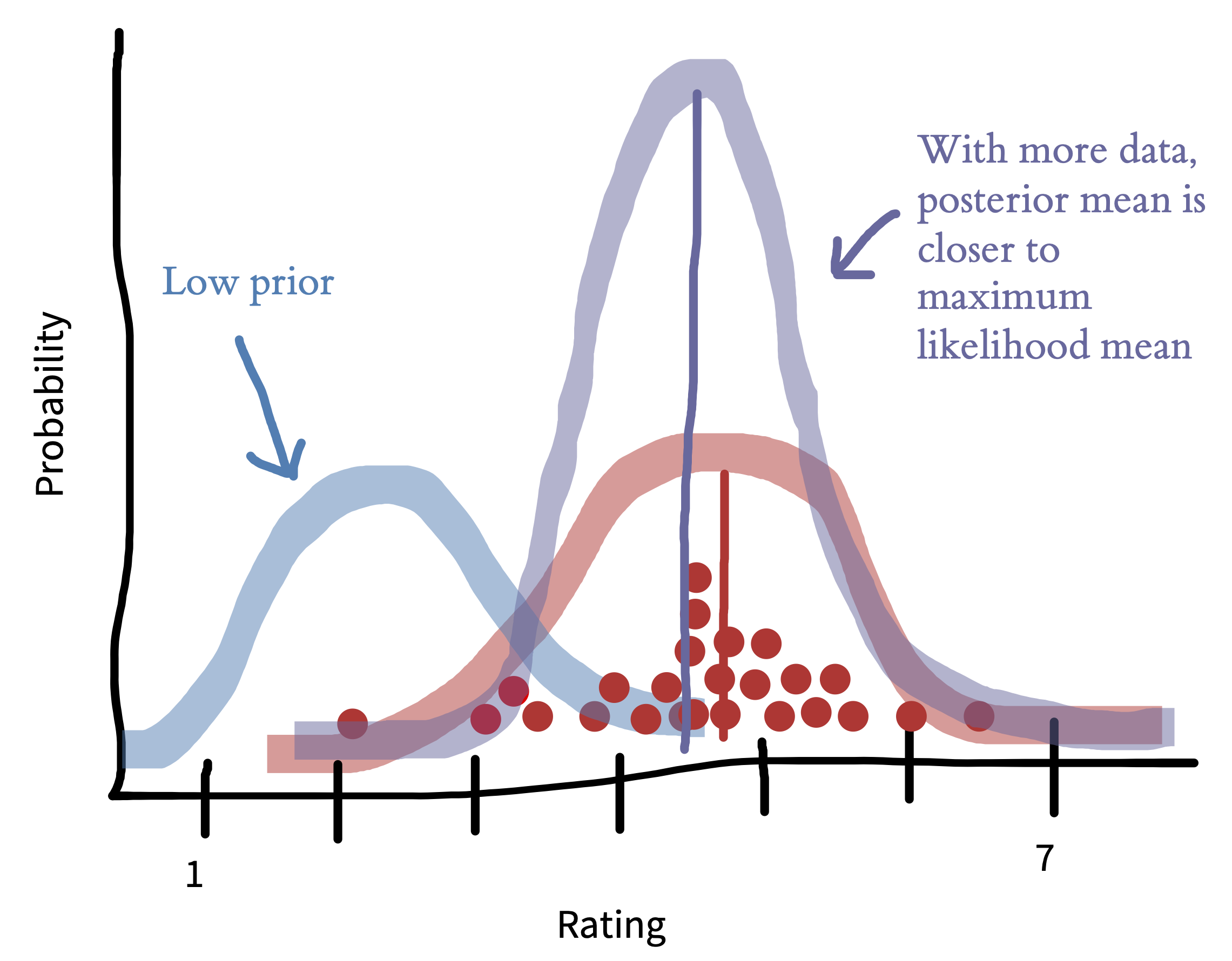
Priors aren’t usually as strong as the one shown above. Figure 5.8 shows how the picture shifts when we have a weaker prior reflecting a flatter, more widely spread belief about the distribution of ratings. Now the posterior mean (purple) is closer to the maximum likelihood mean (red). This situation is more common—the prior encodes a weak assumption that ratings won’t cluster around the ends of the scale.
The effect of the prior is also decreased when you have more data. In figure 5.9, the prior is the same as in figure 5.7, but we have more data. As a result, the posterior distribution is much more peaked and also much closer to the data—the prior makes much less difference.
Bayesian estimation is most important when you have strong beliefs and not a lot of data. That can be a case where you have just a few participants in your experiment, but it’s also good—and perhaps more common—to use Bayesian methods when you have a lot of data, but maybe not that much data about particular units that you care about. For example, you might have a large dataset about the effects of an educational intervention but not that much data about how it affects a particular subgroup. Bayesian estimates and maximum likelihood estimates will exactly coincide either under a flat prior (a prior that makes any value equally likely) or as the amount of data goes to infinity.
5.2 Estimating and comparing effects
We’ve now covered estimating a single parameter (the mean for people who had milk-first tea) using both frequentist and Bayesian methods. But recall that what we really wanted to do was to estimate the causal effect we were interested in, namely the milk-first vs tea-first effect. In this section, we’ll discuss how to estimate the effect, and then how to use effect size measures to compare effects across experiments (as well as some of the pros and cons of doing so).8
8 This method doesn’t have to be used only with a causal effect; it can be any between-group difference. In the current example, we can say with certainty that this effect is a causal one because our experiment uses random assignment.
5.2.1 Estimating the treatment effect
Let’s refer to the causal effect we care about as our treatment effect.9 In practice, estimating \(\beta\) (a parameter describing the treatment effect) is going to be a pretty straightforward extension to what we did before.
9 This is the effect of our manipulation—what we sometimes call an “intervention” as well. “Treatment” is a term that comes from medical statistics but is used more broadly in statistics now.
10 For simplicity, we’re assuming that the standard deviations in each tea group are equal.
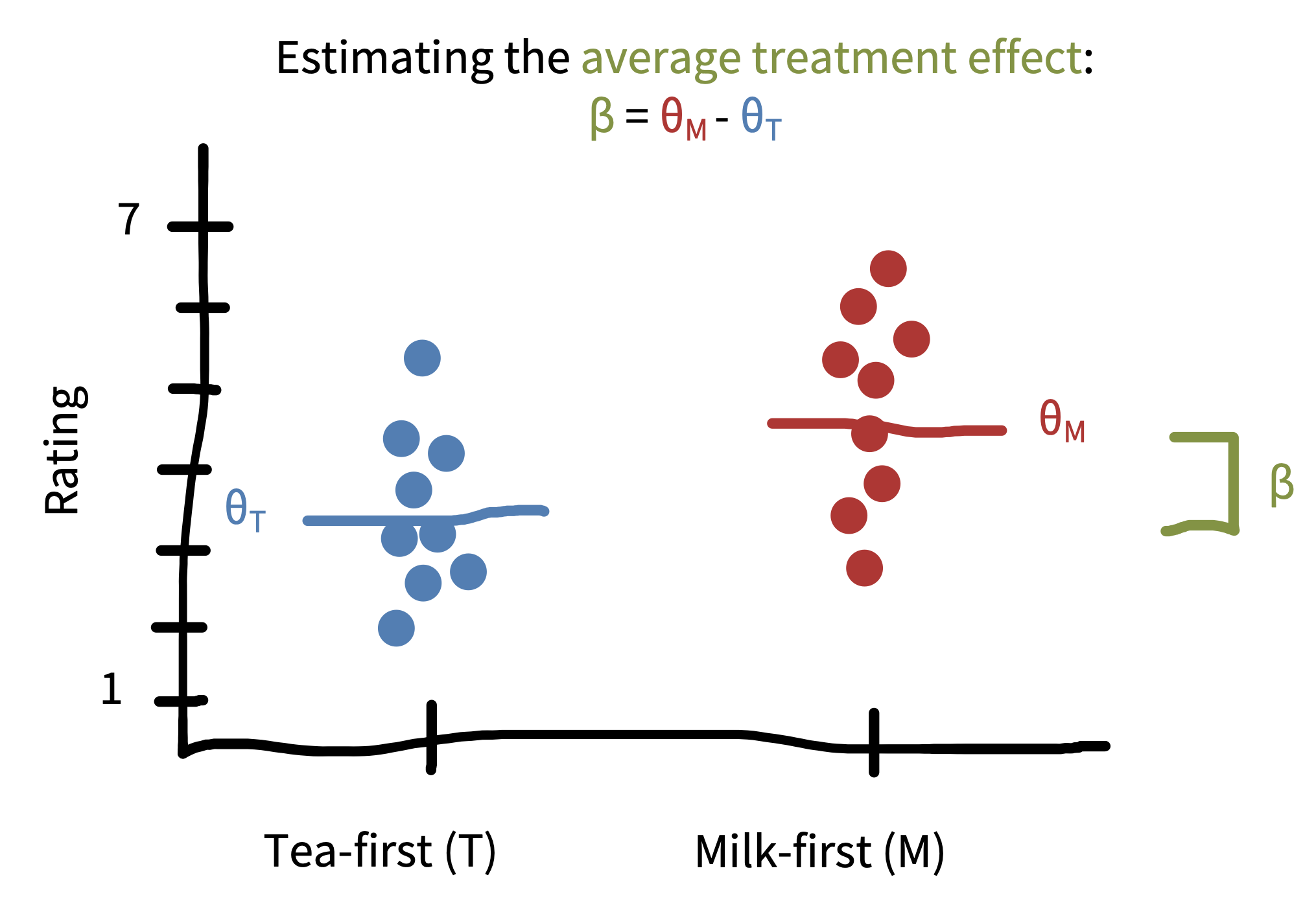
In the maximum likelihood framework, we could posit that ratings in each group (milk-first and tea-first) follow a normal distribution but that these normal distributions might have different means and standard deviations. Extending the notation introduced above, let’s term the parameters for the tea-first group \(\theta_{T}\) (the mean) and \(\sigma\) (the standard deviation). To estimate the treatment effect, we are positing a model in which the milk-first ratings are normally distributed with mean \(\theta_{M} = \theta_{T} + \beta\) and with standard deviation \(\sigma\).10 This equation says that milk-first ratings have the same distribution as tea-first ratings, except that their average is shifted by \(\beta\). Setting our model up this way then lets us compute \(\hat{\beta}\), our estimate of the treatment effect in our sample.
As in the one-sample case (estimating the mean of just the milk-first group), maximum likelihood estimation would then proceed by finding the value of \(\beta\) that makes the data most likely under the assumed model. As you might expect, this estimate \(\widehat{\beta}\) turns out to be simply the difference in sample means, \(\widehat{\theta}_{M}-\widehat{\theta}_{T}\). This difference is pictured in figure 5.10.
In the Bayesian framework, we would again specify a prior \(p(\beta)\) that encodes our prior beliefs about the size and direction of the treatment effect. If we have no prior beliefs at all, then we could specify a flat prior, \(p(\beta) \propto 1\).11 If we believe the treatment effect is likely to favor milk-first pouring (\(\beta>0\)), we could specify that the prior is a normal distribution centered at some positive value (e.g., \(\beta=0.5\)); the standard deviation of this prior would encode how certain we are about our prior beliefs. And, if we have no prior beliefs about the direction of the treatment effect, but we think it is unlikely to be very large, we could specify a normal prior centered at \(0\), which has the effect of “shrinking” the estimates closer to \(0\).12
11 This equation says that the probability of any value of \(\beta\) is “proportional to” \(1\), meaning that it’s constant (“flat”) regardless of what value \(\beta\) takes.
12 The measures of variability that we discuss here account for statistical uncertainty reflecting the fact that we have only a finite sample size. If the sample size were infinite, there would be no uncertainty of this kind. Statistical uncertainty is only one kind of uncertainty, though. A more holistic view of the overall credibility of an estimate should also account for other things outside of the model, like study design issues and bias.
As in our example above, maximum likelihood estimates and Bayesian estimates are going to be pretty similar if we have a lot of data or weak priors. They will only diverge when we have strong priors or relatively little data. The reason we are setting up these two different frameworks, however, is that they provide very different inferential tools, as we’ll see in the next chapter.
5.2.2 Measures of effect size
Once we have measured something, we need to make a decision about how to describe this effect to others. Sometimes we are working with fairly intuitive relationships that are easy to describe. A researcher might say, for example, that people who received milk-first tea drank the tea, on average, five minutes quicker than people who received tea-first tea (i.e., \(\widehat{\beta} = 5\) minutes). Time is measured in units like minutes and seconds and so we have a shared understanding of what five minutes means.
But what about our participants’ ratings of tea quality, which were provided on an arbitrary 7-point rating scale that we devised? What does it mean to that participants who drank milk-first tea rated it 1 point higher than participants who drank tea-first tea (i.e., that \(\widehat{\beta} = 1\) point)? And how is this difference comparable to, for instance, a 1-point change on a scale that has similar anchors (“terrible” and “delicious”) but uses a 100-point rating system?
To provide a common language for describing these relationships, some researchers use standardized effect sizes. A common standardized effect size is Cohen’s \(d\), which provides a standardized estimate of the difference between two means. There are many different ways to calculate Cohen’s \(d\) (Lakens 2013), but all approaches are usually some variant of the following formula:
\[ d = \frac{\theta_{M} - \theta_{T}}{\sigma_{\text{pooled}}} \]
where the difference between means (\(\theta_{T}\) and \(\theta_{M}\)) is divided by the pooled standard deviation \(\sigma_{\text{pooled}}\). Intuitively, what you’re doing is taking the study effect (\(\beta\)) and dividing it—scaling it—by the variation we saw between individuals in the study.13
13 Cohen’s \(d\), also referred to as standardized mean difference (SMD), can be tricky to apply to more complex experimental designs, such as within-participant designs with multiple measurements of each participant. For some guidance on this topic, see Lakens (2013).
Let’s compute this measure for our tea-drinking study. We can just plug in the estimates we see in figure 5.10 and compute the standard deviation of our observed data:
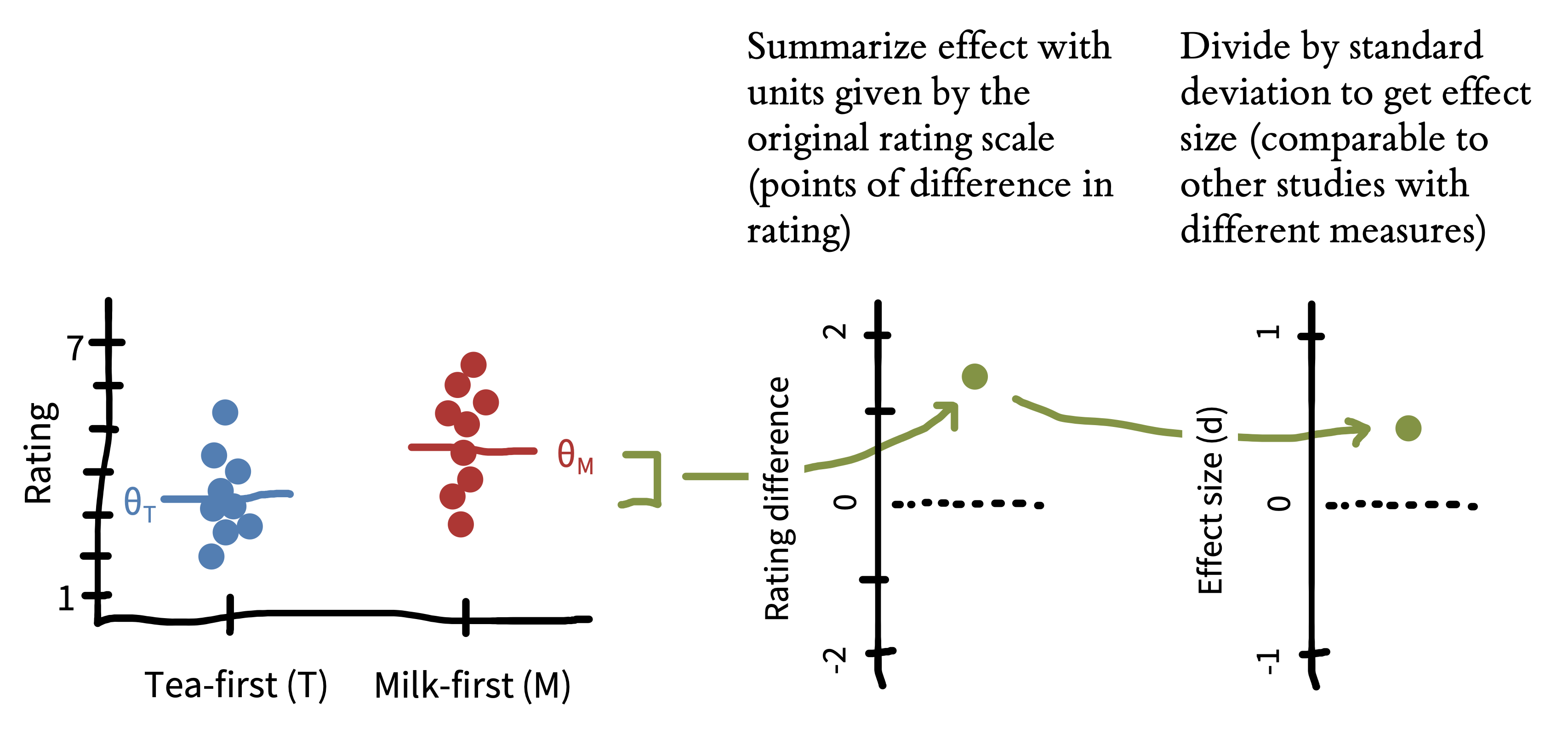
\[\widehat{d} = \frac{\widehat{\theta}_{M} - \widehat{\theta}_{T}}{\widehat{\sigma}_{\text{pooled}}} = \frac{4.5- 3.5}{1.25} = \frac{1}{1.25} = 0.80\] In other words, the effect size of the difference between the two conditions is \(0.8\) standard deviations. This process is shown in figure 5.11.
We previously said that people who drank milk-first tea had quality ratings that were, on average, 1 point higher on a 7-point scale (\(\beta = 1\) point). Cohen’s \(d\) translates the arbitrary units of our rating scale into a unitless that is measured in terms of the variation in the data. You may be wondering: “Why would I ever describe things in terms of standard deviations?” The key benefit is that it allows us to compare the size of the effect between studies that use different measures.
Let’s say that we ran a replication of our tea study with two changes: (1) we studied patrons in a US cafe instead of a UK cafe, and (2) we used a 100-point rating scale instead of a 7-point scale. Imagine that, just as we found that UK participants rated the milk-first tea 1 point higher on a 7-point quality scale, US participants rated the milk-first tea 1 point higher on a 100-point quality scale. It seems clear that these effects are different because of the difference in scale. But how different?
It might at first seem reasonable just to normalize by the length of the scale. So, maybe the UK experimental participants showed a 1/7 rating effect and the US participants showed a 1/100 rating effect. The trouble with this move is that it presupposes that participants from two different populations are using two different scales in exactly the same way! For example, maybe US participants made very clumpy judgments that were mostly centered around 50 (perhaps because of a lack of milk tea experience). Standardized effect sizes get around this kind of issue by scaling according to the variability of the data.
Let’s compute the effect size for the cross-cultural replication. We’ll imagine that participants who drank milk-first tea gave an average rating of 50/100 and participants who drank tea-first tea rated it 49 on average. But if their variability was also relatively lower, perhaps the standard deviation of their ratings was only 5. Using the formula above:
\[\widehat{d}_{\text{US}} = \frac{\widehat{\theta}_{M} - \widehat{\theta}_{T}}{\widehat{\sigma}_{\text{pooled}}} = \frac{50 - 49}{5} = \frac{1}{5}= 0.2\]
A Cohen’s \(d\) of 0.2 means that US cafe patrons rated their tea \(0.2\) standard deviations higher when it was milk-first, much smaller than the \(0.8\) standard deviation difference in the UK patrons.
There are no hard and fast rules for interpreting what makes a big effect or a small effect, but people often refer back to a standard suggested by Cohen (1992). On those standards, \(d = 0.8\) is a “large effect” and \(d = 0.2\) is a “small effect.” But these effect size interpretation norms are somewhat arbitrary. The key point here was that US and UK patrons had the same raw score change in quality ratings (\(\widehat{\beta} = 1\)), and standardizing the differences allowed us to communicate that the difference was larger among the UK patrons.
Cohen’s \(d\) is one of many standardized effect sizes that researchers can use. Just as Cohen’s \(d\) standardizes differences in group means, there are also generalizations that allow for continuous treatment variables or covariate adjustment (e.g., Pearson’s r, as we discuss below; \(r^2\); or \(\eta^2\)). And there is a whole other set of effect-size measures for relationships between binary variables (e.g., odds ratio). We’ll be using effect sizes throughout the book, but we’ll be using Cohen’s \(d\) as our example.14
5.2.3 Pros and cons of standardizing effect sizes
Standardizing effect size helps communicate that a 1-point change on a 7-point scale is not the same as a 1-point change on a 100-point scale. But is it any better to say that the first represents a \(0.8\) standard deviation difference and the second a \(0.08\) standard deviation difference?
Effect sizes allow us to compare results across studies more easily. Across studies, researchers use different measures, different study designs, and different populations. Standardization gives us a “common language” to describe estimated relationships in these varied contexts. This language is helpful when we want to aggregate and compare effects across studies via meta-analysis. And it is also helpful when planning new studies. When trying to figure out how many participants to run in a study, almost all techniques for sample size planning use standardized effect sizes to determine how much data would be needed to reliably detect an effect.
Standardizing effect sizes has limitations, though. For example, if two interventions produce the same absolute change in the same outcome measure, but are studied in different populations in which the variability on the outcome differs substantially, the interventions would produce different standardized mean differences (Baguley 2009) (see the Depth box “Reliability paradoxes!” in chapter 8).
Imagine we conducted our tea experiment again, but this time with decaf tea and focusing on children. Maybe milk-first tea tastes the same amount better than tea-first tea for kids and for adults. But kids are, as a rule, more variable in their responding than adults. This higher level of variability would lead us to observe a smaller effect size in kids vs adults. Recall that our UK adult SD was \(1.25\) and our effect size was \(d = 0.8\). Imagine that children’s SD is \(2.5\). In this scenario, even if tea led to the same 1-point absolute change in ratings among adults and children, the standardized effect size for kids would look half as big:
\[\widehat{d}_{\text{kids}} = \frac{\widehat{\theta}_{M} - \widehat{\theta}_{T}}{\widehat{\sigma}_{\text{pooled}}} = \frac{5- 4}{2.5} = \frac{1}{2.5} = 0.4\]
This example highlights some of the challenges with standardization. If we focused on the fact that both adults and children show a 1-point change in ratings levels (\(\widehat{\beta} = 1\)), we would conclude that milk-first tea ordering is as much better for adults as kids. If we focused on the standardized effect sizes, however, we would conclude that the milk ordering effect is twice as big for adults.
So which is better: Describing raw measures or standardized effect sizes? In general, our response is “Why not both?” But if you were to pick only one, we recommend considering the type of measurement you are using. With measures that yield common measurement units that are likely to be reported in many studies already, use raw scores (Baguley 2009). For example, if your study uses physical units such as milliseconds (e.g., for reaction times) or counts (e.g., for a study tracking an outcome like number of words), these measurements can be quite useful to compare across studies. Reporting raw measurements also can allow you to check whether your measurements make sense—for example, a reaction time of 70 milliseconds is inhumanly fast while a reaction time of 10 seconds might be extremely slow (at least, for many speeded tasks).
In contrast, we recommend using standardized effect sizes for cases where the measurement is relatively unlikely to be comparable with other studies in its original form, or unlikely to be meaningful on its own. For example, reporting the effect of an intervention on raw math test scores is only meaningful if the reader knows how many items are on the test, how difficult it is, and so forth. In such a case where it is hard for a reader to be “calibrated” to the specific measurement units you are using, standardized effect sizes may be the best way to report your finding (Kelley and Preacher 2012).
5.3 Estimating the relationship between variables
15 Remember, this is a correlational relationship, and there’s no causal inference possible here.
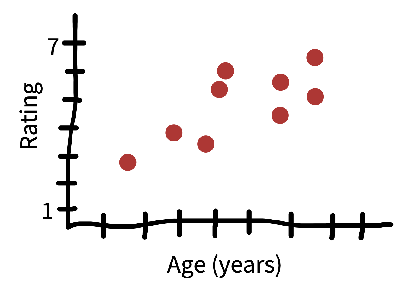
Our focus up until now has been in estimating individual effects, but sometimes we also want to estimate the relationship between two different variables. Extending our example, figure 5.12 shows the relationship between the age of the tea taster and their rating of milk-first tea. It seems that younger people overall like tea less than older people.15 How could we quantify this result?
The first concept we need is covariance. Covariance captures the degree to which we expect two variables to deviate from their means in the same direction. We’re looking at milk-first tea ratings \(M\) and participant ages \(A\). We can write the covariance between these two as
\[\text{cov}(M, A) = E[(M - \theta_M) (A - \theta_A)]\]
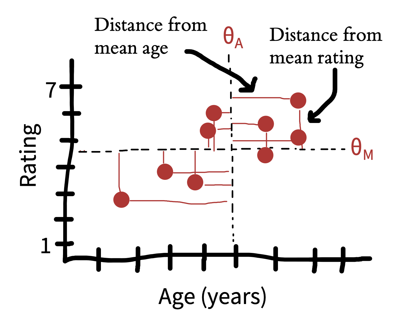
This formula expresses the expected product of how much each observation differs from its expectation (mean) along each variable. Figure 5.13 shows these differences, which are multiplied together for each point to get the covariation.16
16 This looks a little tricky, but it’s actually very related to the basic concepts we’ve already seen. Remember when we introduced the standard deviation, we described it as the expected distance between new samples from a distribution and the mean of that distribution. The covariance is very related: the standard deviation is just \(\sqrt{\text{cov}(X,X)}\), in other words, the square root of the covariance of a variable with itself.
This covariance number gives us an estimate of how much age and ratings covary, but its units are a bit funny: it’s hard to know what to make of an expected deviation of 1 point-year. We can do a simple trick to standardize its units and make it into a wonderful form of effect size—the correlation coefficient (denoted \(r\)). Remember that to create effect sizes above, we divided by the standard deviation of the variable. Here all we have to do is divide by the standard deviation of both variables.
\[r_{M,A} = \frac{\text{cov}(M,A)}{\sigma_M \sigma_A}\] In other words, the correlation between two variables is the standardized covariation.
The correlation coefficient is the most ubiquitous measure of association between variables. It ranges between \(-1\), where two variables covary in exactly the opposite direction, to \(1\), when two variables covary perfectly. A correlation means that there is no association between two variables. A correlation of \(-1\) or \(1\) doesn’t mean that the variables have the same scale, however: it just means that they “move together.”
Critically, a correlation is an effect size. Correlations can be compared across different measures and different studies (including both experimental and observational studies), making it a very valuable scale-free comparison tool.17
17 This section has described one way of looking at a correlation coefficient: as standardized covariation. For a great discussion of all the different ways of thinking about correlations, see Lee Rodgers and Nicewander (1988).
5.4 Chapter summary: Estimation
In this chapter, we introduced the idea of estimating both individual measurements and treatment effects from observed data. These ideas are simple but they lay the foundations for hypothesis testing and modeling (our next two chapters). Further, we set up the distinction between Bayesian and frequentist approaches, which we will expand in the next chapter since these traditions provide different inferential tools.
In this chapter you learned about estimation, and in this book more generally, we have argued that the goal of an experiment is to provide a maximally precise estimate of a causal effect. Psychology as a field has often been criticized for focusing too much on inference and too little on estimation. Find an article in the journal Psychological Science that reports on an experiment or series of experiments and read the abstract. Does it mention an estimate of any particular quantity? What might be the benefits of reporting estimates in the study abstract?
Try the same exercise with a paper in the New England Journal of Medicine or Journal of the American Medical Association. Find a paper and check if there is a mention of any specific quantity being estimated. (We suspect there will be!) Consider this contrast between the medical article and the psychology article. What do you make of this difference between fields?
A great narrative introduction to the history and practice of statistics: Salsburg, Daniel. (2002). The Lady Tasting Tea: How Statistics Revolutionized Science in the Twentieth Century. Macmillan.
An open-source statistics textbook that follows a similar approach as chapters 5—7: Poldrack, Russell A. (2024). Statistical Thinking for the 21st Century. Available free online at https://statsthinking21.org.